From Simulated Ore to £63.7m at Risk: How a Supply-Chain Lakehouse Computes Its Numbers

Most "supply chain analytics" demos start with a clean sales table and end with a sales chart. This one starts earlier and ends later — earlier, because the data is simulated rather than downloaded, so it behaves like a real supply chain instead of just looking like one; and later, because the goal isn't a chart, it's a decision: how much to stock, which suppliers could halt production, and how much revenue is exposed if they do.

This post walks the whole chain. First, how the data is generated so that sales, inventory, purchase orders, and goods receipts all agree with one another. Then how the medallion layers refine it. And finally, how every headline number — a 66% error reduction, £14.2m of safety stock, a supplier risk score of 80/100, £63.7m of revenue at risk — is actually computed. No number here is asserted; each one is derived, and I'll show the derivation.

Part 1 — Generating data that behaves like a supply chain

The temptation with synthetic data is to generate each table independently: random sales here, random purchase orders there. That produces tables that look plausible in isolation but contradict each other — a stockout in the sales table with no corresponding dip in inventory, a goods receipt for an order that was never placed. Any analytics built on top inherits those contradictions.

So instead of generating tables, I generated a system and let the tables fall out of it. The core is a day-by-day inventory simulation, run independently for each of the 60 SKUs across each of 4 distribution centres, over two years of daily history. Each day, four things happen in order: arriving shipments are received, demand is realised, sales are capped by what's on the shelf, and a replenishment order fires if stock has fallen too low.

Demand itself isn't random noise. Each SKU has a baseline rate shaped by its category, then modulated by weekly seasonality (hardware sells on weekdays, apparel on weekends), annual seasonality (electronics peak before the holidays), a slow trend, and occasional promotions that lift demand 1.5–3×. About a quarter of SKUs are intermittent slow-movers whose demand is mostly zero with sporadic spikes — the kind of series that breaks naive forecasters. Daily demand is drawn from a Poisson distribution around that shaped rate.

The replenishment side is where the resilience story is seeded. Each SKU is sourced from a primary supplier, and each of the 8 suppliers has its own lead-time distribution and reliability. When stock crosses its reorder point, an order is placed; it arrives after a lead time sampled from that supplier's distribution — with a small probability of a disruption spike that multiplies the lead time several-fold. Reliable domestic suppliers deliver in about a week with little variance; flaky overseas ones average a month with a long, ugly tail.

Because the simulation is one connected loop, the tables it emits reconcile by construction. A stockout in fact_sales corresponds to depleted on-hand in fact_inventory, which triggered a row in fact_purchase_orders, which arrived late in fact_goods_receipts. That coherence is what makes the downstream analytics meaningful rather than decorative.

Two deliberately planted signals matter most:

Censored demand. When demand exceeds on-hand stock, the customer wants more than you can sell them. The sales record shows only what shipped — the rest of the demand is invisible. Across the dataset this happens on about 7.3% of SKU-location-days. The simulation records the true underlying demand in a hidden column so we can later check whether we can recover it; in a real system that column wouldn't exist, which is exactly the point.

Lead-time variability by supplier. The realised order-to-receipt gaps separate cleanly by reliability tier:

Tier	Mean lead time	Std dev	Worst case
Reliable	7.7 days	3.6	32 days
Variable	21.4 days	6.9	90 days
Flaky	30.3 days	19.3	154 days

And concentration: 41 of the 60 SKUs are single-sourced, with no backup supplier — the population that makes disruption expensive.

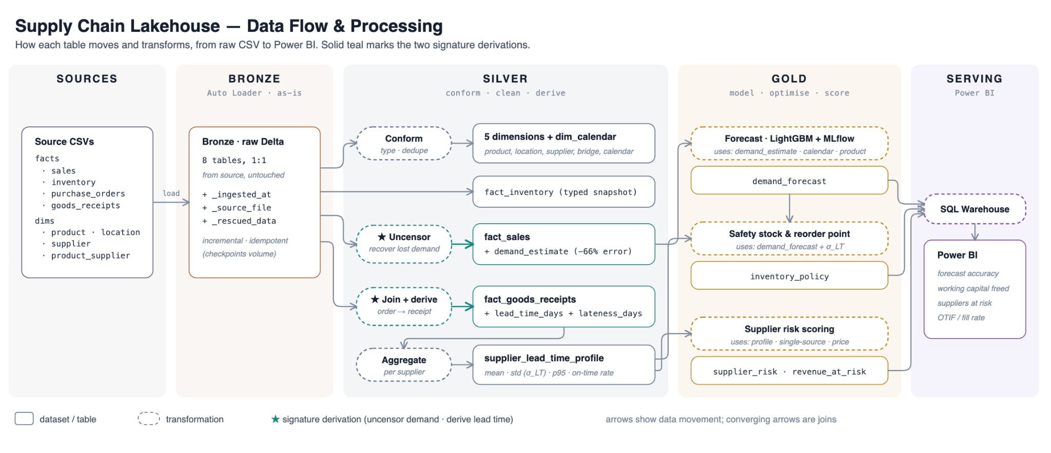
Part 2 — Refining the data (Bronze → Silver)

Bronze is deliberately boring. Each raw CSV lands as a Delta table essentially as-is, with lineage columns recording where each row came from and when it was loaded. Nothing is cleaned, because Bronze's job is to be a faithful, replayable record of what the source systems said. If a number looks wrong three weeks later, you trace it back here.

Silver is where the data starts to reflect reality rather than just what the systems happened to record. It conforms and types the dimensions, builds a calendar, and performs the two derivations the whole project depends on.

Recovering demand that stockouts hid

Here's the first headline number and how it's earned. On stockout days, units_sold is capped by on-hand stock, so it under-reports true demand. Feeding those censored zeros and caps straight into a forecaster teaches it to under-predict exactly the items that stock out most — a quietly destructive, self-reinforcing bias.

The fix doesn't require the hidden ground truth. For each SKU and location, we compute a baseline expected demand from the days that weren't stockouts, broken down by day of week to preserve the weekly rhythm. On a stockout day, we lift the censored figure up to that baseline:

baseline = sales[sales.is_stockout == 0] \
    .groupby(["product_id", "location_id", "day_of_week"]).units_sold.mean()

demand_estimate = where(is_stockout,
                        max(units_sold, baseline),   # recover the lost demand
                        units_sold)                  # otherwise trust the record

To prove it works, we compare both the raw and corrected series against the hidden true demand, on the ~12,800 stockout days only:

• Using raw units_sold, mean absolute error is 47.4 units, and it's pure downward bias — you can never sell more than you stocked, so every error is an under-count.
• Using the corrected demand_estimate, error drops to 16.2 units, and the bias shrinks from −47.4 to −11.1.

That's a 66% reduction in error — 1 − 16.2/47.4. Put plainly: left uncorrected, demand on stockout days is under-counted by roughly 100%, and that bias would propagate into every forecast and every safety-stock figure downstream.

Deriving what suppliers actually do

The second derivation joins each goods receipt back to its purchase order and computes the realised lead time as the gap between order and receipt, plus lateness against the promised date. Crucially, the analytics trust observed behaviour, not the supplier's nominal promise — the entire resilience story lives in the gap between the two. Aggregated per supplier, this becomes a lead-time profile (mean, standard deviation, 95th percentile, on-time rate) that feeds everything in Gold.

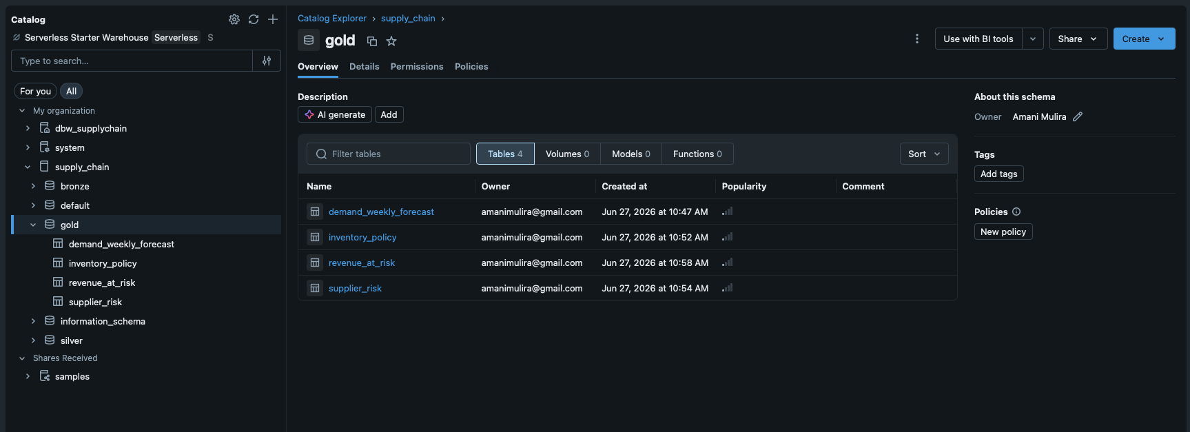
Part 3 — Turning data into decisions (Gold)

Gold is four computations. Only the first is machine learning; the rest are deterministic math on top of the Silver signals.

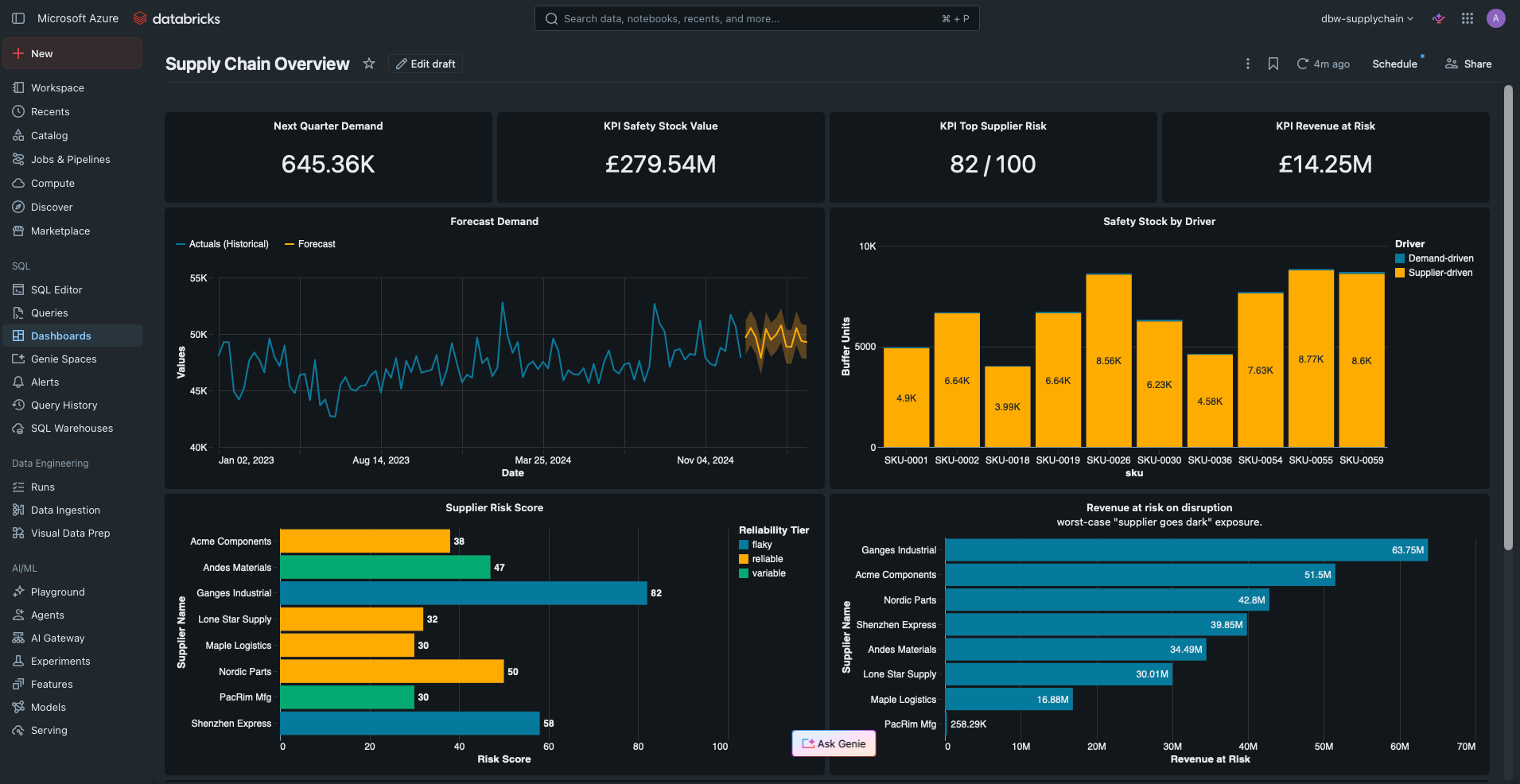
Demand forecast — 3.3% MAPE

Weekly demand is aggregated from the corrected series, then modelled as a linear trend plus a week-of-year seasonal factor, projected 13 weeks ahead with an 80% prediction band from the residual spread. To report an honest accuracy figure, we back-test: fit on everything except the last 13 weeks, predict them, and compare. The mean absolute percentage error comes out at 3.3% — low, as you'd expect for aggregate demand, which is far smoother than any single SKU. The forward forecast sums to about 645,000 units for the coming quarter. (At per-SKU grain you'd swap in a gradient-boosted or per-series model; the aggregate is what drives the headline chart.)

Safety stock — and what it's really protecting against

Safety stock is the buffer that absorbs uncertainty while you wait for a replenishment. The textbook formula, accounting for both demand and lead-time variability, is:

SS = z · √( LT · σ_D²  +  D² · σ_LT² )

where z is the service-level factor (1.65 for 95%), D and σ_D are mean and standard deviation of daily demand, and LT and σ_LT are the mean and standard deviation of lead time. Reorder point is then D · LT + SS.

What makes this interesting is the two terms under the square root. The first, LT · σ_D², is the buffer you hold because demand is unpredictable. The second, D² · σ_LT², is the buffer you hold because your supplier is unpredictable. Splitting safety stock into these two components tells you, per SKU, whether the fix is better forecasting or a more reliable supplier.

A revealing pattern falls out: for high-volume SKUs the D² term is large, so even modest supplier variability dominates the buffer. The biggest-buffer items are overwhelmingly supplier-driven — their inventory is a tax on unreliable lead times, not volatile demand. Valued at cost, the recommended safety stock across the catalogue totals £14.2m, and the split tells you which suppliers are quietly forcing you to hold it.

Supplier risk — a single comparable score

Risk isn't just unreliability; it's unreliability weighted by what's at stake. The score combines four normalised factors per supplier: lead-time variability (30%), lateness, i.e. one minus on-time rate (25%), single-source concentration (20%), and revenue exposure (25%). Each factor is min-max scaled across the eight suppliers, weighted, and expressed out of 100.

The model surfaces Ganges Industrial at 80/100 — the worst supplier, and correctly so: it has the highest lead-time standard deviation (19.3 days), poor on-time performance, several single-source SKUs, and meaningful revenue flowing through it. The scoring needs no hand-labelling; it's a direct, defensible function of observed behaviour. Note too that a reliable supplier can still score moderately if enough revenue and single-source SKUs concentrate on it — risk is exposure times likelihood, and the score captures both.

Revenue at risk — the disruption headline

The final question is the bluntest: if a supplier disappears tomorrow, how much revenue stops? Multi-source SKUs can fail over to their backup; single-source SKUs cannot. So for each supplier we sum the annualised revenue of the SKUs that are single-sourced to it — the revenue that genuinely halts.

Across the catalogue, £279.5m of annual revenue sits behind single-source suppliers with no failover. The single worst exposure is Ganges Industrial at £63.7m across 5 SKUs — if it goes dark, that revenue stalls until those SKUs are re-sourced. The quietly uncomfortable finding is the runner-up: a reliable supplier carrying £51.5m of single-source revenue. It rarely fails, but if it ever did, the blast radius is enormous — a concentration risk that a reliability score alone would never flag.

Securing the lakehouse — identity, least privilege, and governance

None of the above is worth much if the data underneath it isn't locked down. The security model here is worth a section of its own, because it follows a principle that's easy to state and easy to get wrong: the data never moves, and nothing holds a key.

The data never moves because Databricks reads it in place, in the customer's own Azure Data Lake Storage account. There are no copies shipped to a third-party service and no extracts emailed around — which means securing the project is about controlling identity and access to one location, not chasing copies across systems.

Nothing holds a key because access is brokered through a managed identity rather than a stored secret. An Access Connector for Azure Databricks is issued a system-assigned identity in Microsoft Entra ID, and that identity is what reaches the storage account. There is no account key, no SAS token, and no connection string sitting in a notebook or a config file to be leaked, committed to git, or rotated on a schedule. The single most common cause of cloud data breaches — a leaked credential — is designed out rather than guarded against.

That identity is granted exactly one thing: the Storage Blob Data Contributor role, scoped to the storage account. It can read and write data and nothing else — no ability to change account settings, delete the resource, or touch other services. This is least privilege in its plainest form, and it has a useful property: revoke that single role assignment and every read stops instantly, with no secret to also hunt down and invalidate.

Identity itself lives in Microsoft Entra ID, so users and groups are governed centrally. Multi-factor authentication and conditional-access policies apply at that layer, before anyone reaches Databricks at all, and the first account administrator must be an Entra Global Administrator — there's no separate, parallel set of credentials to manage for the data platform.

Inside the platform, Unity Catalog is the governance broker, and this is where access control gets fine-grained. Reaching the storage isn't enough on its own; a user needs an explicit grant on the external location and volume that map to a storage path, so people can't wander into arbitrary buckets even from inside a notebook. Permissions are expressed as ordinary GRANT/REVOKE statements over a three-level catalog.schema.table namespace, which makes the medallion layers a natural security boundary: analysts can be given read access to gold only, while engineers work across bronze, silver, and gold. Unity Catalog also records column- and table-level lineage and access logs, so every figure on the dashboard can be traced back to its source table, and every read can be traced back to a user.

Underneath all of that, the usual protections still apply. Azure Storage encrypts data at rest by default, with the option to bring customer-managed keys via Azure Key Vault for organisations that require control of the encryption keys themselves; traffic moves over TLS in transit; and for a hardened deployment the storage account can be placed behind a firewall with private endpoints so it has no public exposure and is reachable only from the Databricks workspace's network.

The result is defence in depth that reads as a single chain: Entra ID authenticates who, the scoped RBAC role authorises what in storage, Unity Catalog governs which data each person sees and logs every access, and encryption protects the bytes at rest and in flight. Each link is independent, and the most failure-prone one — a long-lived secret — simply isn't part of the design.

The through-line

Read together, the numbers tell one story. A bias planted in the raw data (censored demand) would have quietly corrupted every figure downstream, until a simple, ground-truth-free correction removed two-thirds of the error. The same flaky supplier surfaces independently as both the highest risk score and the largest disruption exposure — two different computations pointing at the same throat to protect. And the safety-stock split reveals that much of the inventory on the balance sheet exists not because customers are fickle, but because suppliers are.

Every figure in this post is computed, not assumed, and the data is synthetic — but the logic is production-shaped. Swap the simulated CSVs for a company's real order, inventory, and receipt feeds, and the same pipeline produces the same kind of answers, with the same chain of reasoning behind each one.

Appendix — the notebooks

The three pieces of code behind Parts 1 and 2 are reproduced in full below, so the post is self-contained and reproducible. The Databricks notebooks use the # COMMAND ---------- cell separators, so they import directly as notebooks.

1 · Data generation — generate_supply_chain_data.py

The inventory simulation that emits the eight internally-consistent source tables. Run locally (pandas/numpy); seeded, so it reproduces exactly.

"""
Synthetic supply chain dataset generator.

Produces an internally consistent set of source-system tables for a demand-
forecasting + inventory-positioning + supplier-resilience project. The core is a
day-by-day inventory simulation per (product, location): demand depletes on-hand,
purchase orders fire when the inventory position crosses a reorder point, and
goods receipts arrive after a supplier-specific lead time that occasionally spikes
(disruption). This makes sales, inventory snapshots, POs, and receipts all agree
with one another instead of being independent random tables.

Outputs (CSV, ready to land in a Bronze layer):
    dim_product.csv
    dim_location.csv
    dim_supplier.csv
    product_supplier.csv         (sourcing map; flags single-source SKUs)
    fact_sales.csv               (daily demand; includes ground-truth true_demand)
    fact_inventory_snapshot.csv  (end-of-day on-hand per SKU/location)
    fact_purchase_orders.csv
    fact_goods_receipts.csv
"""

import numpy as np
import pandas as pd
from datetime import date, timedelta

rng = np.random.default_rng(42)
OUT = "/mnt/user-data/outputs"

START = date(2023, 1, 1)
DAYS = 730                       # 2 years of daily history
dates = [START + timedelta(days=i) for i in range(DAYS)]
dow = np.array([d.weekday() for d in dates])          # 0=Mon .. 6=Sun
doy = np.array([d.timetuple().tm_yday for d in dates]) # 1..366

# ---------------------------------------------------------------- locations
locations = [
    (1, "DC-North",   "North",   "US"),
    (2, "DC-South",   "South",   "US"),
    (3, "DC-West",    "West",    "US"),
    (4, "DC-Central", "Central", "US"),
]
loc_scale = {1: 1.2, 2: 1.0, 3: 0.8, 4: 1.1}
dim_location = pd.DataFrame(locations, columns=["location_id", "location_name", "region", "country"])

# ---------------------------------------------------------------- suppliers
# id, name, country, region, lt_mean, lt_std, disruption_prob, disruption_mult, tier
suppliers = [
    (1, "Acme Components",   "US", "Domestic", 5,  1.0, 0.010, 1.8, "reliable"),
    (2, "Nordic Parts",      "DE", "Europe",   12, 2.5, 0.020, 2.0, "reliable"),
    (3, "PacRim Mfg",        "CN", "Asia",     28, 5.0, 0.050, 2.5, "variable"),
    (4, "Shenzhen Express",  "CN", "Asia",     24, 6.0, 0.080, 3.0, "flaky"),
    (5, "Lone Star Supply",  "US", "Domestic", 6,  1.5, 0.015, 1.8, "reliable"),
    (6, "Andes Materials",   "CL", "LatAm",    20, 4.0, 0.040, 2.2, "variable"),
    (7, "Ganges Industrial", "IN", "Asia",     26, 7.0, 0.100, 3.5, "flaky"),
    (8, "Maple Logistics",   "CA", "Domestic", 7,  1.2, 0.010, 1.6, "reliable"),
]
sup_cols = ["supplier_id", "supplier_name", "country", "region",
            "lead_time_mean_days", "lead_time_std_days",
            "disruption_prob", "disruption_mult", "reliability_tier"]
dim_supplier = pd.DataFrame(suppliers, columns=sup_cols)
SUP = {s[0]: dict(zip(sup_cols[1:], s[1:])) for s in suppliers}
domestic_suppliers = [1, 5, 8]
overseas_suppliers = [2, 3, 4, 6, 7]

# ---------------------------------------------------------------- categories
# category -> (annual_amp, peak_doy, weekly_factors[Mon..Sun])
CATS = {
    "Electronics": (0.35, 330, [1.00, 1.00, 1.00, 1.05, 1.15, 1.25, 1.10]),  # holiday peak
    "Hardware":    (0.15, 120, [1.15, 1.15, 1.10, 1.10, 1.05, 0.70, 0.55]),  # weekday/B2B
    "Consumables": (0.10, 200, [1.00, 1.00, 1.00, 1.00, 1.05, 1.05, 0.95]),  # steady
    "Apparel":     (0.40, 350, [0.90, 0.90, 0.95, 1.00, 1.15, 1.35, 1.20]),  # weekend + winter
    "Tools":       (0.30, 150, [1.10, 1.10, 1.10, 1.10, 1.10, 1.00, 0.60]),  # spring/summer
}
cat_list = list(CATS.keys())

# ---------------------------------------------------------------- products
N_PRODUCTS = 60
prod_rows = []
prod_supplier_rows = []
prod_params = {}   # product_id -> dict of demand params

for pid in range(1, N_PRODUCTS + 1):
    cat = cat_list[(pid - 1) % len(cat_list)]
    amp, peak, weekly = CATS[cat]
    # base demand: mix of fast and slow movers; ~25% intermittent slow movers
    is_intermittent = rng.random() < 0.25
    if is_intermittent:
        base = float(rng.uniform(0.3, 2.5))        # sparse demand
    else:
        base = float(rng.uniform(8, 60))           # regular movers
    unit_cost = round(float(rng.uniform(3, 250)), 2)
    margin = float(rng.uniform(0.25, 0.65))
    unit_price = round(unit_cost * (1 + margin), 2)
    trend_slope = float(rng.uniform(-0.15, 0.35))  # 2-year drift, mostly growth
    abc = "A" if base > 35 else ("B" if base > 12 else "C")
    prod_rows.append((pid, f"SKU-{pid:04d}", f"{cat} item {pid}", cat,
                      unit_cost, unit_price, abc, int(is_intermittent)))

    # ---- sourcing: primary supplier, ~40% multi-source with a secondary
    primary = int(rng.choice(overseas_suppliers + domestic_suppliers))
    sources = [primary]
    if rng.random() < 0.40:
        # secondary from a different region where possible
        candidates = [s for s in (domestic_suppliers + overseas_suppliers)
                      if SUP[s]["region"] != SUP[primary]["region"]]
        secondary = int(rng.choice(candidates))
        sources.append(secondary)
    single_source = int(len(sources) == 1)
    for rank, sid in enumerate(sources, start=1):
        prod_supplier_rows.append((pid, sid, rank, 1 if rank == 1 else 0, single_source))

    # ---- precompute daily demand lambda (product level, before location scale)
    weekly_arr = np.array([weekly[d] for d in dow])
    annual_arr = 1 + amp * np.cos(2 * np.pi * (doy - peak) / 365.0)
    trend_arr = 1 + trend_slope * (np.arange(DAYS) / DAYS)
    promo_arr = np.ones(DAYS)
    # 2-4 promo windows/year, each 5-10 days, lift 1.5-3x
    n_promos = rng.integers(4, 9)
    for _ in range(n_promos):
        start = int(rng.integers(0, DAYS - 10))
        length = int(rng.integers(5, 11))
        promo_arr[start:start + length] *= float(rng.uniform(1.5, 3.0))
    lam = base * weekly_arr * annual_arr * trend_arr * promo_arr
    lam = np.clip(lam, 0.01, None)
    prod_params[pid] = dict(cat=cat, base=base, is_intermittent=is_intermittent,
                            lam=lam, promo=(promo_arr > 1.0).astype(int),
                            primary=primary)

dim_product = pd.DataFrame(prod_rows, columns=[
    "product_id", "sku", "product_name", "category",
    "unit_cost", "unit_price", "abc_class", "is_intermittent"])
product_supplier = pd.DataFrame(prod_supplier_rows, columns=[
    "product_id", "supplier_id", "source_rank", "is_primary", "is_single_source"])

# ---------------------------------------------------------------- simulation
sales_rows = []
inv_rows = []
po_rows = []
receipt_rows = []
po_counter = 0

def sample_lead_time(sid):
    """Lead time in days, with a fat-tailed disruption spike for flaky suppliers."""
    s = SUP[sid]
    lt = rng.normal(s["lead_time_mean_days"], s["lead_time_std_days"])
    if rng.random() < s["disruption_prob"]:
        lt *= s["disruption_mult"]
    return max(1, int(round(lt)))

for pid in range(1, N_PRODUCTS + 1):
    p = prod_params[pid]
    sid = p["primary"]
    lt_mean = SUP[sid]["lead_time_mean_days"]
    for lid, lname, region, country in locations:
        scale = loc_scale[lid]
        mean_daily = max(0.05, p["base"] * scale)
        # simple order-up-to policy sized off mean demand and lead time
        review_period = 14
        reorder_point = mean_daily * (lt_mean + 5)          # cover lead time + buffer
        order_up_to = reorder_point + mean_daily * review_period
        on_hand = float(order_up_to)                         # start full
        pending = []                                         # list of (arrival_idx, qty)
        on_order = 0.0

        for t in range(DAYS):
            d = dates[t]
            # 1) receive anything arriving today
            still = []
            for arr_idx, qty in pending:
                if arr_idx == t:
                    on_hand += qty
                    on_order -= qty
                else:
                    still.append((arr_idx, qty))
            pending = still

            # 2) realise demand (Poisson); intermittent SKUs gate to mostly zero
            lam_t = p["lam"][t] * scale
            if p["is_intermittent"]:
                demand = int(rng.poisson(lam_t)) if rng.random() < 0.35 else 0
            else:
                demand = int(rng.poisson(lam_t))
            sold = min(demand, int(on_hand))
            stockout = int(demand > on_hand)
            on_hand -= sold
            sales_rows.append((d, pid, lid, sold, demand, p["promo"][t], stockout))
            inv_rows.append((d, pid, lid, int(on_hand), int(on_order)))

            # 3) reorder if inventory position has dropped to/below reorder point
            position = on_hand + on_order
            if position <= reorder_point:
                qty = int(round(order_up_to - position))
                if qty > 0:
                    po_counter += 1
                    po_id = f"PO{po_counter:07d}"
                    lt = sample_lead_time(sid)
                    arrival = t + lt
                    promised = d + timedelta(days=lt_mean)
                    receipt_date = d + timedelta(days=lt)
                    po_rows.append((po_id, sid, pid, lid, d, qty, promised))
                    if arrival < DAYS:
                        pending.append((arrival, qty))
                        on_order += qty
                        receipt_rows.append((po_id, sid, pid, lid, receipt_date, qty, lt))
                    else:
                        # PO placed but not yet received within the horizon
                        receipt_rows.append((po_id, sid, pid, lid, None, 0, None))

fact_sales = pd.DataFrame(sales_rows, columns=[
    "order_date", "product_id", "location_id",
    "units_sold", "true_demand", "promo_flag", "stockout_flag"])
fact_inventory = pd.DataFrame(inv_rows, columns=[
    "snapshot_date", "product_id", "location_id", "on_hand_units", "on_order_units"])
fact_po = pd.DataFrame(po_rows, columns=[
    "po_id", "supplier_id", "product_id", "location_id",
    "order_date", "qty_ordered", "promised_date"])
fact_receipt = pd.DataFrame(receipt_rows, columns=[
    "po_id", "supplier_id", "product_id", "location_id",
    "receipt_date", "qty_received", "actual_lead_time_days"])

# ---------------------------------------------------------------- write
tables = {
    "dim_product": dim_product,
    "dim_location": dim_location,
    "dim_supplier": dim_supplier,
    "product_supplier": product_supplier,
    "fact_sales": fact_sales,
    "fact_inventory_snapshot": fact_inventory,
    "fact_purchase_orders": fact_po,
    "fact_goods_receipts": fact_receipt,
}
for name, df in tables.items():
    df.to_csv(f"{OUT}/{name}.csv", index=False)

# ---------------------------------------------------------------- summary
print("Rows written:")
for name, df in tables.items():
    print(f"  {name:28s} {len(df):>8,d} rows  x {df.shape[1]} cols")

stockout_rate = fact_sales["stockout_flag"].mean()
censored = (fact_sales["true_demand"] > fact_sales["units_sold"]).mean()
print(f"\nStockout days:           {stockout_rate:6.2%} of SKU-location-days")
print(f"Censored-demand days:    {censored:6.2%} (true demand > units sold)")

lt = fact_receipt.dropna(subset=["actual_lead_time_days"]).merge(
    dim_supplier[["supplier_id", "supplier_name", "reliability_tier"]], on="supplier_id")
print("\nActual lead time by supplier reliability tier:")
print(lt.groupby("reliability_tier")["actual_lead_time_days"]
        .agg(["mean", "std", "max"]).round(1).to_string())

ss = product_supplier.groupby("product_id")["is_single_source"].first()
print(f"\nSingle-source SKUs:      {int(ss.sum())} of {N_PRODUCTS}")
print(f"Total purchase orders:   {len(fact_po):,d}")

2 · Loading — 02_bronze_autoloader.py (Databricks notebook)

Auto Loader incrementally ingests each CSV into a raw Delta table in Unity Catalog, adding lineage. Re-runnable and idempotent.

# Databricks notebook source
# MAGIC %md
# MAGIC # Bronze ingestion — Auto Loader
# MAGIC Incrementally loads each raw CSV into a Bronze Delta table in Unity Catalog.
# MAGIC Each source table lives in its own folder under the raw_files volume; one Auto
# MAGIC Loader stream watches each folder and writes to its own table. Re-runs are
# MAGIC incremental and idempotent (checkpoints track what's been seen), so this is
# MAGIC safe to schedule. Bronze keeps the data essentially as-is and adds lineage;
# MAGIC all real cleaning happens later in Silver.

# COMMAND ----------

from pyspark.sql.functions import current_timestamp, col

CATALOG = "supply_chain"
BRONZE  = "bronze"
VOLUME_ROOT     = f"/Volumes/{CATALOG}/{BRONZE}/raw_files"
CHECKPOINT_ROOT = f"/Volumes/{CATALOG}/{BRONZE}/checkpoints"
TABLES = ["dim_product", "dim_location", "dim_supplier", "product_supplier",
          "fact_sales", "fact_inventory_snapshot", "fact_purchase_orders", "fact_goods_receipts"]

# the checkpoint path must be a real Unity Catalog volume before any stream writes to it
spark.sql(f"CREATE VOLUME IF NOT EXISTS {CATALOG}.{BRONZE}.checkpoints")
spark.sql(f"USE CATALOG {CATALOG}")
spark.sql(f"USE SCHEMA {BRONZE}")

# COMMAND ----------

# Each source table must sit in its own folder (raw_files/<table>/<table>.csv) so its
# stream only ever sees files that share one schema. If the CSVs were uploaded flat into
# the volume root, this moves each into its own folder first.
present = {f.name.rstrip("/") for f in dbutils.fs.ls(VOLUME_ROOT)}
for t in TABLES:
    if f"{t}.csv" in present:
        dbutils.fs.mkdirs(f"{VOLUME_ROOT}/{t}")
        dbutils.fs.mv(f"{VOLUME_ROOT}/{t}.csv", f"{VOLUME_ROOT}/{t}/{t}.csv")
        print(f"moved {t}.csv -> {t}/")

# COMMAND ----------

def directory_has_files(path: str) -> bool:
    try:
        return len(dbutils.fs.ls(path)) > 0
    except Exception:
        return False

def ingest(table: str):
    source = f"{VOLUME_ROOT}/{table}"
    ckpt   = f"{CHECKPOINT_ROOT}/{table}"
    target = f"{CATALOG}.{BRONZE}.{table}"
    if not directory_has_files(source):
        print(f"  skipping {table}: no files at {source}")
        return
    stream = (
        spark.readStream.format("cloudFiles")
        .option("cloudFiles.format", "csv")
        .option("header", "true")
        .option("cloudFiles.inferColumnTypes", "true")
        .option("cloudFiles.schemaLocation", ckpt)
        .option("rescuedDataColumn", "_rescued_data")   # malformed/unexpected fields land here, never dropped
        .load(source)
        .withColumn("_source_file", col("_metadata.file_path"))   # Bronze lineage
        .withColumn("_ingested_at", current_timestamp())
    )
    (stream.writeStream
        .option("checkpointLocation", ckpt)
        .option("mergeSchema", "true")
        .trigger(availableNow=True)        # process everything available, then stop
        .toTable(target)
        .awaitTermination())
    print(f"  loaded -> {target}")

for t in TABLES:
    print(f"Ingesting {t} ...")
    ingest(t)
print("\nBronze ingestion complete.")

# COMMAND ----------

# MAGIC %md ## Verify — row counts should match the generated dataset

# COMMAND ----------

for t in TABLES:
    n = spark.table(f"{CATALOG}.{BRONZE}.{t}").count()
    print(f"{t:28s} {n:>9,d} rows")

# Expected: fact_sales 175,200 | fact_inventory_snapshot 175,200
#           fact_purchase_orders 11,136 | fact_goods_receipts 11,136
#           dim_product 60 | product_supplier 79 | dim_supplier 8 | dim_location 4

3 · Transformation — 03_silver_transforms.py (Databricks notebook)

Conforms the dimensions, builds a calendar, and performs the two signature derivations: uncensoring demand and deriving observed supplier lead times.

# Databricks notebook source
# MAGIC %md
# MAGIC # Silver layer — conform, clean, derive
# MAGIC Reads Bronze Delta tables and produces typed, conformed Silver tables.
# MAGIC The two transformations that matter most:
# MAGIC  * **fact_sales** — estimate *uncensored* demand on stockout days (the raw
# MAGIC    `units_sold` is capped by on-hand and systematically under-counts demand).
# MAGIC  * **fact_goods_receipts** — derive *actual* lead time and lateness by joining
# MAGIC    each receipt back to its purchase order. This is the raw material for safety
# MAGIC    stock (σ_LT) and supplier risk scoring.

# COMMAND ----------

CATALOG = "supply_chain"
spark.sql(f"USE CATALOG {CATALOG}")

from pyspark.sql import functions as F

def bronze(name):
    return spark.table(f"{CATALOG}.bronze.{name}")

def write_silver(df, name):
    (df.write.mode("overwrite").option("overwriteSchema", "true")
       .saveAsTable(f"{CATALOG}.silver.{name}"))
    print(f"  wrote silver.{name:28s} {df.count():>9,d} rows")

# COMMAND ----------

# MAGIC %md ## Dimensions — type, dedupe, enrich

# COMMAND ----------

# dim_product: cast, derive margin economics (needed later for revenue-at-risk)
dim_product = (bronze("dim_product")
    .select(
        F.col("product_id").cast("int"),
        "sku", "product_name", "category",
        F.col("unit_cost").cast("double"),
        F.col("unit_price").cast("double"),
        "abc_class",
        F.col("is_intermittent").cast("int"))
    .withColumn("unit_margin", F.round(F.col("unit_price") - F.col("unit_cost"), 2))
    .withColumn("margin_pct",  F.round((F.col("unit_price") - F.col("unit_cost")) / F.col("unit_price"), 3))
    .dropDuplicates(["product_id"]))
write_silver(dim_product, "dim_product")

dim_location = (bronze("dim_location")
    .select(F.col("location_id").cast("int"), "location_name", "region", "country")
    .dropDuplicates(["location_id"]))
write_silver(dim_location, "dim_location")

# disruption_prob / mult are the data's nominal generative params; the resilience
# layer should trust OBSERVED behaviour (the lead-time profile below), not these.
dim_supplier = (bronze("dim_supplier")
    .select(
        F.col("supplier_id").cast("int"),
        "supplier_name", "country", "region",
        F.col("lead_time_mean_days").cast("double").alias("nominal_lead_time_mean"),
        F.col("lead_time_std_days").cast("double").alias("nominal_lead_time_std"),
        "reliability_tier")
    .dropDuplicates(["supplier_id"]))
write_silver(dim_supplier, "dim_supplier")

# sourcing bridge: which suppliers feed which SKUs; single-source flag
product_supplier = (bronze("product_supplier")
    .select(
        F.col("product_id").cast("int"),
        F.col("supplier_id").cast("int"),
        F.col("source_rank").cast("int"),
        F.col("is_primary").cast("int"),
        F.col("is_single_source").cast("int"))
    .dropDuplicates(["product_id", "supplier_id"]))
write_silver(product_supplier, "product_supplier")

# COMMAND ----------

# dim_calendar: built here, not ingested — gives forecasting its time features
dim_calendar = (spark.sql(
        "SELECT explode(sequence(to_date('2023-01-01'), to_date('2024-12-31'), interval 1 day)) AS date")
    .withColumn("year",         F.year("date"))
    .withColumn("month",        F.month("date"))
    .withColumn("day_of_month", F.dayofmonth("date"))
    .withColumn("day_of_week",  F.dayofweek("date"))          # 1=Sun .. 7=Sat
    .withColumn("week_of_year", F.weekofyear("date"))
    .withColumn("quarter",      F.quarter("date"))
    .withColumn("is_weekend",   F.col("day_of_week").isin(1, 7).cast("int")))
write_silver(dim_calendar, "dim_calendar")

# COMMAND ----------

# MAGIC %md
# MAGIC ## fact_sales — uncensor demand
# MAGIC On stockout days `units_sold` is capped by on-hand, so it under-reports true
# MAGIC demand. We estimate the lost demand from a day-of-week baseline built only from
# MAGIC non-stockout days, and keep both the raw and corrected series.

# COMMAND ----------

sales = (bronze("fact_sales")
    .select(
        F.to_date("order_date").alias("order_date"),
        F.col("product_id").cast("int"),
        F.col("location_id").cast("int"),
        F.col("units_sold").cast("int"),
        F.col("promo_flag").cast("int"),
        F.col("stockout_flag").cast("int").alias("is_stockout"),
        # ground truth exists only because the data is synthetic — never available
        # in a real system; kept solely to validate the correction.
        F.col("true_demand").cast("int").alias("true_demand_ground_truth"))
    .withColumn("dow", F.dayofweek("order_date")))

baseline = (sales.filter("is_stockout = 0")
    .groupBy("product_id", "location_id", "dow")
    .agg(F.avg("units_sold").alias("baseline_dow")))

fact_sales = (sales
    .join(baseline, ["product_id", "location_id", "dow"], "left")
    .withColumn("demand_estimate",
        F.when(F.col("is_stockout") == 1,
               F.greatest(F.col("units_sold"), F.round("baseline_dow").cast("int")))
         .otherwise(F.col("units_sold")))
    .withColumn("demand_estimate", F.coalesce("demand_estimate", "units_sold"))
    .drop("dow", "baseline_dow"))
write_silver(fact_sales, "fact_sales")

# COMMAND ----------

fact_inventory = (bronze("fact_inventory_snapshot")
    .select(
        F.to_date("snapshot_date").alias("snapshot_date"),
        F.col("product_id").cast("int"),
        F.col("location_id").cast("int"),
        F.col("on_hand_units").cast("int"),
        F.col("on_order_units").cast("int")))
write_silver(fact_inventory, "fact_inventory")

# COMMAND ----------

fact_po = (bronze("fact_purchase_orders")
    .select(
        "po_id",
        F.col("supplier_id").cast("int"),
        F.col("product_id").cast("int"),
        F.col("location_id").cast("int"),
        F.to_date("order_date").alias("order_date"),
        F.col("qty_ordered").cast("int"),
        F.to_date("promised_date").alias("promised_date")))
write_silver(fact_po, "fact_purchase_orders")

# COMMAND ----------

# MAGIC %md
# MAGIC ## fact_goods_receipts — derive actual lead time
# MAGIC Join each receipt to its PO. The gap between order and receipt is the realised
# MAGIC lead time; the gap against the promised date is lateness. These feed σ_LT in the
# MAGIC safety-stock formula and the supplier on-time score.

# COMMAND ----------

receipts_raw = (bronze("fact_goods_receipts")
    .select(
        "po_id",
        F.col("supplier_id").cast("int"),
        F.col("product_id").cast("int"),
        F.col("location_id").cast("int"),
        F.to_date("receipt_date").alias("receipt_date"),
        F.col("qty_received").cast("int")))

fact_receipt = (receipts_raw
    .join(fact_po.select("po_id", "order_date", "promised_date"), "po_id", "left")
    .withColumn("lead_time_days",     F.datediff("receipt_date", "order_date"))
    .withColumn("lateness_days",      F.datediff("receipt_date", "promised_date"))
    .withColumn("is_on_time",        (F.col("lateness_days") <= 0).cast("int"))
    .withColumn("is_received",        F.col("receipt_date").isNotNull().cast("int")))
write_silver(fact_receipt, "fact_goods_receipts")

# COMMAND ----------

# Supplier lead-time profile: the OBSERVED distribution per supplier.
# This is the resilience backbone — mean/std drive safety stock, the tail (p95) and
# on-time rate drive the risk score.
supplier_lead_time_profile = (fact_receipt
    .filter("is_received = 1")
    .groupBy("supplier_id")
    .agg(
        F.count("*").alias("n_receipts"),
        F.round(F.avg("lead_time_days"), 1).alias("lead_time_mean"),
        F.round(F.stddev("lead_time_days"), 1).alias("lead_time_std"),
        F.expr("percentile_approx(lead_time_days, 0.5)").alias("lead_time_p50"),
        F.expr("percentile_approx(lead_time_days, 0.95)").alias("lead_time_p95"),
        F.max("lead_time_days").alias("lead_time_max"),
        F.round(F.avg("is_on_time"), 3).alias("on_time_rate"))
    .join(dim_supplier.select("supplier_id", "supplier_name", "reliability_tier"),
          "supplier_id", "left"))
write_silver(supplier_lead_time_profile, "supplier_lead_time_profile")

# COMMAND ----------

# MAGIC %md ## Validate — the correction and the lead-time signal

# COMMAND ----------

# 1) Censored-demand correction vs ground truth, on stockout days only.
v = spark.table(f"{CATALOG}.silver.fact_sales").filter("is_stockout = 1")
v.select(
    F.count("*").alias("stockout_days"),
    F.round(F.mean(F.abs(F.col("units_sold")      - F.col("true_demand_ground_truth"))), 2).alias("MAE_raw"),
    F.round(F.mean(F.abs(F.col("demand_estimate") - F.col("true_demand_ground_truth"))), 2).alias("MAE_corrected"),
).show()

# 2) Observed lead-time profile — flaky suppliers should stand out on std and p95.
spark.table(f"{CATALOG}.silver.supplier_lead_time_profile") \
    .orderBy(F.desc("lead_time_std")).show(truncate=False)

4 · Dashboard datasets — 05_dashboard_queries.sql

The SQL behind each AI/BI dashboard tile. Every query reads from the Gold marts (produced by 04_gold_marts.py); the note in [brackets] marks the visualization type each dataset drives.

-- ============================================================================
-- 05_dashboard_queries.sql
-- One dataset per dashboard tile. In the AI/BI dashboard editor: Data tab ->
-- Create from SQL -> paste a query -> name the dataset as noted. Then add a
-- widget on the Canvas and bind it to that dataset with the visualization type
-- shown in [brackets].
-- ============================================================================

-- ───────────────────────── KPI counters [Counter] ──────────────────────────
-- dataset: kpi_next_quarter_demand   [Counter] value = next_quarter_demand
SELECT SUM(forecast) AS next_quarter_demand
FROM supply_chain.gold.demand_weekly_forecast
WHERE is_forecast;

-- dataset: kpi_safety_stock_value    [Counter] value = safety_stock_value, prefix £
SELECT SUM(safety_stock_value) AS safety_stock_value
FROM supply_chain.gold.inventory_policy;

-- dataset: kpi_top_supplier_risk     [Counter] value = top_risk_score (suffix /100)
SELECT MAX(risk_score) AS top_risk_score
FROM supply_chain.gold.supplier_risk;

-- dataset: kpi_revenue_at_risk       [Counter] value = revenue_at_risk, prefix £
SELECT SUM(revenue_at_risk) AS revenue_at_risk
FROM supply_chain.gold.revenue_at_risk;

-- ───────────────────── Forecast demand [Line chart] ────────────────────────
-- X = week_start,  Y = actual AND forecast (two series).
-- Optionally add lower/upper as faint lines for the confidence band.
SELECT week_start, actual, forecast, lower, upper
FROM supply_chain.gold.demand_weekly_forecast
ORDER BY week_start;

-- ────────────── Safety stock by driver [Bar chart, stacked] ─────────────────
-- X = sku,  Y = buffer_units,  Color/Group = driver,  Layout = Stack.
WITH t AS (
  SELECT sku,
         SUM(ss_demand_component)   AS demand_driven,
         SUM(ss_supplier_component) AS supplier_driven,
         SUM(safety_stock)          AS total_ss
  FROM supply_chain.gold.inventory_policy
  GROUP BY sku
  ORDER BY total_ss DESC
  LIMIT 10
)
SELECT sku, 'Demand-driven'   AS driver, demand_driven   AS buffer_units FROM t
UNION ALL
SELECT sku, 'Supplier-driven' AS driver, supplier_driven AS buffer_units FROM t;

-- ─────────────────── Supplier risk score [Bar chart] ───────────────────────
-- X = risk_score,  Y = supplier_name (horizontal),  Color = reliability_tier.
SELECT supplier_name, risk_score, reliability_tier,
       lead_time_mean, on_time_rate, n_single_source
FROM supply_chain.gold.supplier_risk
ORDER BY risk_score DESC;

-- ──────────────── Revenue at risk on disruption [Bar chart] ─────────────────
-- X = revenue_at_risk,  Y = supplier_name (horizontal). Sort desc; the top bar
-- is the worst-case "supplier goes dark" exposure.
SELECT supplier_name, revenue_at_risk, n_single_source_skus
FROM supply_chain.gold.revenue_at_risk
ORDER BY revenue_at_risk DESC;

-- ─────────── (optional) Detail table behind the policy [Table] ──────────────
SELECT sku, category, supplier_name, mean_daily_demand, lead_time_mean,
       safety_stock, reorder_point, safety_stock_value, is_single_source
FROM supply_chain.gold.inventory_policy
ORDER BY safety_stock_value DESC
LIMIT 200;